Department of Scientific Computing    Institute for Numerical Simulation    University of Bonn

Documentation

Download

Programming References

Bug Reports / Suggestions

FAQ

Authors

Discretization of Operators & Algorithms

The tensor product structure of the anisotropic wavelets leads to a very simple structure of algorithms. Similar to the multivariate Fourier transform, which is performed by nested univariate transforms along the lines and the rows, the algorithms for the basis transforms, evaluation of differential operators, quadratures and so on can be decomposed into the nested application of the respective univariate operator along a particular coordinate direction. As an example take the discretization of the partial derivative with respect to $x$.

Consider a finite dimensional approximation to a function u : $\sum_{({\bf l,t}) \in {\cal{T}}} u_{\bf l,t} \psi_{\bf l,t} \approx u$. We want to find an approximation to the first derivative w.r.t. x: $\sum_{({\bf l,t}) \in {\cal{T}}} v_{\bf l,t} \psi_{\bf l,t} \approx \partial_x u$. It is convenient to describe the principal idea for the two-dimensional case. Then, the multiindices read ${\bf l}=(l_0,l_1)$ and ${\bf t}=(t_0,t_1)$. The index set ${\cal{T}}$ is decomposed into 'lines' along the x-coordinate direction

$${\cal{T}}_{l_1,t_1} := \{(l_0,t_0): ({\bf l,t}) \in {\cal{T}}\}$$

i.e.

$${\cal{T}} = \bigcup_{(l_1,t_1) \in {\cal{T}}_0}   \bigcup_... ...al{T}}_0 :=\{(l_1,t_1): {\cal{T}}_{l_1,t_1} \neq \emptyset \}$$

Then

$$\partial_x \sum_{({\bf l,t}) \in {\cal{T}}} u_{\bf l,t} \psi... ...{l_1,t_1}} v_{\bf l,t} \psi_{l_0,t_0}(x) } \psi_{l_1,t_1}(y)$$

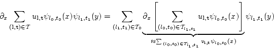
The derivative of the term in the brackets [...] can be discretized using finite differences. The main steps are

1. inverse wavelet transform to obtain the nodal values on an univariate grid with points depending on ${\cal{T}}_{l_1,t_1}$
2. application of the univarite finite difference scheme
3. wavelet transform with respect to the particular coordinate direction

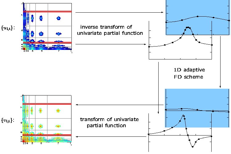
The figure below is a graphical sketch of the scheme for the 2D case. The squares on the left hand side represent the wavelet space with a certain arrangement of the indices/wavelet coefficients. The coloured entries are the coefficients for the indices from ${\cal{T}}$ (the colour corresponds to their magnitude). The white region corresponds to indices which are not in ${\cal{T}}$. In each step just one line (marked by the red bars; we have shown two different lines in this example) of coefficients is read and inverse transformed. This yields the nodal values of an univariate partial function on a (non-uniform) grid. The grid is dependent on the particular line. To these values the finite difference scheme is applied. Then, a wavelet transform yields the coefficients of the result. This repeats for all lines. Vertical lines would be read/written for derivatives with respect to the y-coordinate direction. An analysis of the resulting consistency error is given in [3] for regular sparse grids and in [5] for general adaptive grids.

In the same fashion, a multivariate inverse Interpolet transform is performed. First by an inverse transform along $x$ and then along $y$. Note, this simple scheme for the transform works for Interpolets only, and not for e.g. Lifting Interpolets or the Daubechies wavelets! To explain why is a longer story ;-) !