 |
|
Next: Runtime Consistency Checks Up: Boundary Conditions Previous: Dirichlet boundary conditions
Neumann boundary conditions
Again, we consider the two-dimensional case, only. The extension to higher dimensions follows the same lines,
but is, however, not really straightforward.
Assume the Neumann values on the face
![]() are given by means of
are given by means of ![]() .
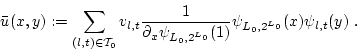
Similar to the Dirichlet case we can define a simple function
.
Similar to the Dirichlet case we can define a simple function ![]() which takes the Neumann values
which takes the Neumann values ![]() on
on ![]() via the wavelet
coefficients
via the wavelet
coefficients ![]() of
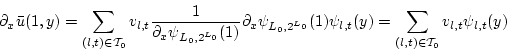
of ![]() . Then,
. Then,
Clearly,
For a level 5 regular sparse or full grid, Neumann values as shown below(left), the resulting function ![]() looks like
looks like
The above situation represents a very simple case, as there are no other faces with Neumann BC. To explain the difficulties
involved then, we consider the case of Neumann BC ![]() at the face
at the face
![]() and
and ![]() at
at
![]() , respectively. The Neumann values are shown below:
, respectively. The Neumann values are shown below:
A simple idea to obtain ![]() would be to generate two functions
would be to generate two functions ![]() and
and ![]() in the same fashion as in (5.3) which take the Neumann BC on just
in the same fashion as in (5.3) which take the Neumann BC on just ![]() and
and ![]() , respectively,
and to add these two functions.
In general
, respectively,
and to add these two functions.
In general
![]() does not take the desired boundary values, e.g.
does not take the desired boundary values, e.g.
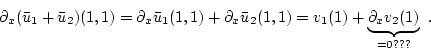
If
The idea ist to find a function ![]() which is non zero in a neighbourhood of the critical point
which is non zero in a neighbourhood of the critical point ![]() only.
In the vicinity of
only.
In the vicinity of ![]() , this function behaves like
, this function behaves like
One easily verifies that
Now, the clou is that under the additional constraint that
the modified Neumann-values
Remark: (5.3) is simply the necessary condition on
the Neumann values to allow for the existence of a function ![]() which is
two times differentiable in (1,1).
which is
two times differentiable in (1,1).
In the high dimensional case we proceed in a similar fashion. First, some auxiliary functions
are computed which are defined in the vicinity of e.g. corners only where several Neumann faces touch.
E.g. in the three dimensional case and a Neumann-Neumann-Neumann-corner these functions look like
As you see, the whole thing gets more and more involved the higher the dimension is. For this reason the current implementation of AdaptiveData<D>::SetBoundaryValueFunction handles two- and three-dimensional cases, only.
Next: Runtime Consistency Checks Up: Boundary Conditions Previous: Dirichlet boundary conditions koster 2003-07-29