Department of Scientific Computing    Institute for Numerical Simulation    University of Bonn

Documentation

Download

Programming References

Bug Reports / Suggestions

FAQ

Authors

AdaptiveData

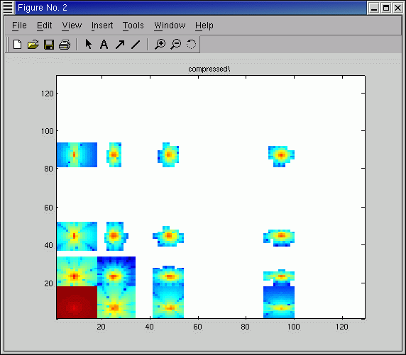
We continue with adaptive representations of a function. First the (anisotropic) wavelet coefficients computed in the WT.cc example are read, and used to initialize an AdaptiveData. Then, we do a simple threshold which retains only those wavelets in the adaptive basis whose wavelet coefficients are larger than 1e-4 by their absolute value plus some neighbours in space and level. Finally the compressed wavelet representation as well as nodal values of the compressed function are written. The source to this example is Sources/Examples/AD.cc. You can compile it by make AD in the Examples directory.

see the code AD.cc

Visualize the results in MATLAB by (AWFD/Sources/Examples/ad.m)

C=ReadUDF('../../Data/Test/C') ;
C1=ReadUDF('../../Data/Test/C1') ;
c=C1.a ;
for i=1:129;for j=1:129; if (c(i,j)==0) c(i,j)=nan ;end;end;end
figure(1); pcolor(log(abs(C.a ))); shading flat;title 'original'
figure(2); pcolor(log(abs(c ))); shading flat;title 'compressed'
A=ReadUDF('../../Data/Test/A') ;
A1=ReadUDF('../../Data/Test/A1') ;
figure(3); surf(A.a) ;shading flat; title 'original'
figure(4); surf(A1.a) ;shading flat; title 'compressed'

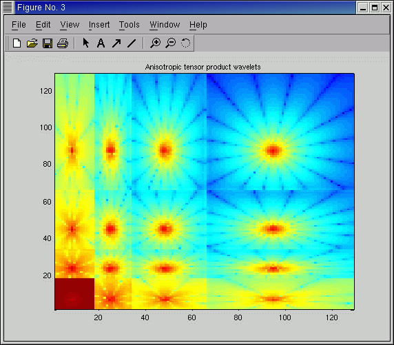
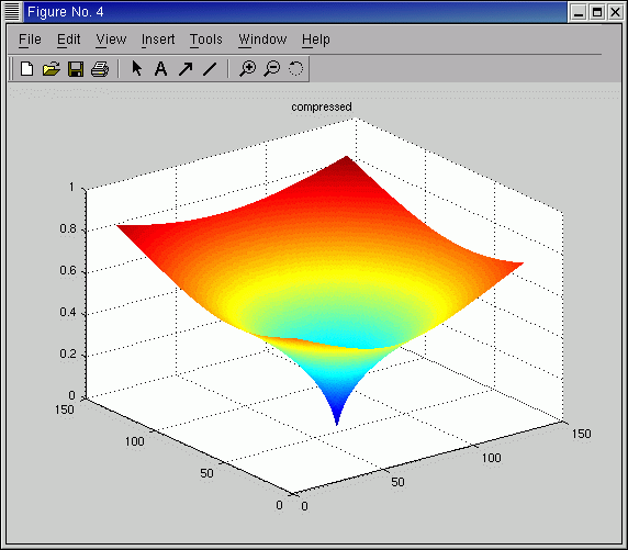
You should get the following four figures. Figures 1 and 2 show the wavelet coefficients. The white regions in figure 2 correspond to neglected wavelet coefficients. Figures 3 and 4 show the nodal values of the original and the compressed functions. Although significantly less degrees of freedom have been used, you hardly see any difference.