 |
|
Next: Adaptive Solution of a Up: Examples Previous: AdaptiveData
Calculation of Partial Derivatives
In the next example we show how to evaluate partial derivatives. First the wavelet coefficients
computed by WT and AD are read and the uniform and adaptive data structures are initialized.
Then the first derivative w.r.t the x-coordinate direction is evaluated by means of 4th order
finite differences. Nodal values of the results are written to an UDF file.
The source to this example is Sources/Examples/PD.cc. You can compile it by
make PD in the Examples directory.
see the code PD.cc
Visualize the result in MATLAB by (AWFD/Sources/Examples/pd.m)
Ax =ReadUDF('../../Data/Test/Ax') ;
A1x=ReadUDF('../../Data/Test/A1x') ;
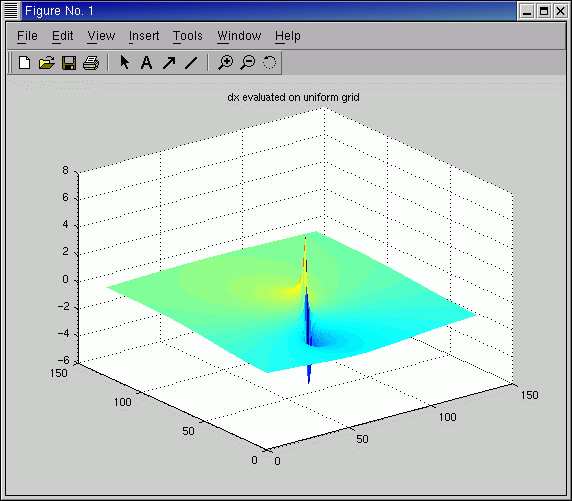
figure(1); surf(Ax.a ); shading flat;title 'dx evaluated on uniform grid'
figure(2); surf(A1x.a); shading flat;title 'dx evaluated on adaptive grid'
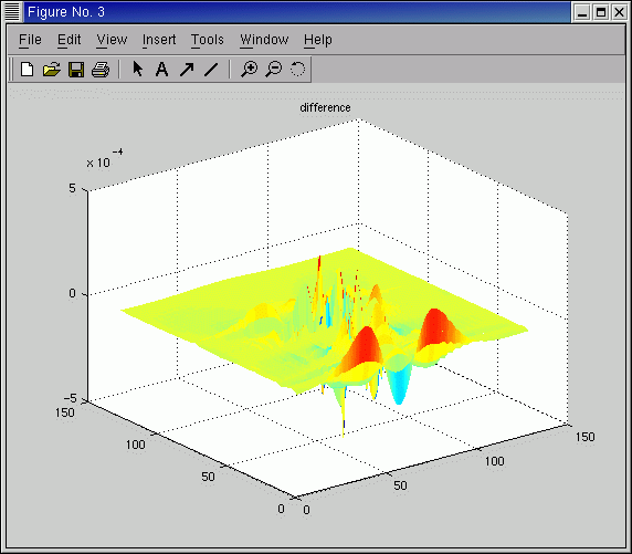
figure(3); surf(Ax.a-A1x.a); shading flat;title 'difference'
You should get the following three figures. Figures 1 and 2 show the nodal values of the derivative. Figure 3 shows the differences. They are very small.


koster 2003-07-29