 |
|
Next: Solution of the Navier-Stokes Up: Examples Previous: Calculation of Partial Derivatives
Adaptive Solution of a Poisson Equation
In this example a Poisson problem with Dirichlet and/or Neumann boundary conditions is solved.
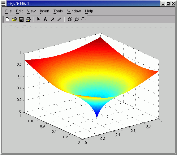
The solution is the spiky function from our first example.
The non-homogeneous Dirichlet or Neumann-values are put on the right hand side to obtain a problem
with homogeneous boundary conditions.
The common solve-refine-cycle is employed to successively increase accuracy.
Refinement is controlled by a threshold criterion.
In former experiments we observed oscillating index sets, that means indices which where
included in the adaptive basis, because the corresponding wavelet coefficient was large,
were thrown out in the next cycle, and after that again included.
To avoid this behaviour we mark all indices whose coefficients
fulfilled the threshold criterion at least for one time. These are kept in the index set for all times.
The source to this example is Sources/Examples/PO.cc. You can compile it by make PO in the Examples directory.
see the code PO.cc
Visualize the results in MATLAB by (AWFD/Sources/Examples/po.m)
U=ReadUDF('../../Data/Test/U') ;
figure(1) ;
[x,y]=meshgrid(U.x{1},U.x{2}) ;
q=[1:8:1025] ; surf(x(q,q),y(q,q),U.a(q,q)) ; shading flat;
figure(2) ;
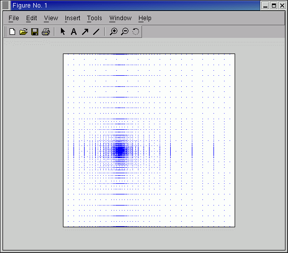
G=ReadSparse('../../Data/Test/U.adp', 0 ) ;
m=2^G.L ;
g=sparse(G.index(:,1)+1 , m-(G.index(:,2)-1) +1 , G.val) ;
spy(g',0.1) ;
set(gca,'XTick',[],'YTick',[], 'XTickLabel',[], 'YTickLabel',[]) ;
xlabel('') ;
You should get the following two figures. Figure 2 shows the distribution of points for the adaptive grid of the final solution.


Next: Solution of the Navier-Stokes Up: Examples Previous: Calculation of Partial Derivatives koster 2003-07-29