Next: Utilities Up: Scene description file Previous: parameter Contents
Objects
Objects are used to describe the geometry of the simulation domain and to specify initial and boundary conditions. There are four basic object types, box, sphere, cylinder and halfspace. Additional geometries and obstacles can be created with the CSG operations union, difference and intersection. There exists one restriction for obstacle cells, namely two opposite faces are not allowed to touch fluid cells.
As already mentioned in section ![]() , objects are just another type of blocks.
The commands given in table
, objects are just another type of blocks.
The commands given in table ![]() can be used inside any object-block.
can be used inside any object-block.
Now we describe the differences between the object-types.
- box:
- The command box defines the box
![$ [X_1,X_2]\times[Y_1,Y_2]\times[Z_1,Z_2]$](img209.png) except one of the keywords north, south, west, east, top or
bottom is given. In this case, the box is the appropriate ''wall'' (see figure
except one of the keywords north, south, west, east, top or
bottom is given. In this case, the box is the appropriate ''wall'' (see figure ![[*]](file:/usr/share/latex2html/icons/crossref.png) ):
):
north 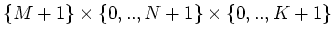
south 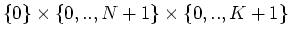
west 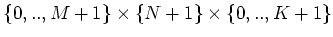
east 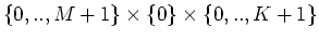
top 
bottom 
- sphere:
- The command sphere defines the ellipsoid which touches all faces of the box
defined by coords.
The main axes are parallel to the coordinate axes.
- cylinder:
- In the same way, cylinder defines a cylinder whose rotation axis is defined
by one of the commands x, y or z.
- halfspace:
- The command halfspace defines the set of cells
where
 are given by the command
hesse < ,
, ,
, >,
>,
and is the middle of the corresponding cell
  .
.
- poly:
- The command poly defines a polytope bounded by polygons. The points are
specified using the command
points ,<
,< ,
, ,
, >,
>, ,<
,< ,
, ,
, > .
> .
The first point indexed with 0. After defining points, the polygons have to be be specified using the command
vertices, ,
, ,...,
,...,
where is the total number of indices (including control indices  ).
One polygon is defined by enumerating the points in clockwise or counterclockwise order, where
the first point has to be enumerated once again as last point. Then this series is finished
with index . The following example defines a cube:
).
One polygon is defined by enumerating the points in clockwise or counterclockwise order, where
the first point has to be enumerated once again as last point. Then this series is finished
with index . The following example defines a cube:
poly { points 8,<0.0,0.0,0.0>, <1.0,0.0,0.0>, <1.0,1.0,0.0>, <0.0,1.0,0.0>, <0.0,0.0,1.0>, <1.0,0.0,1.0>, <1.0,1.0,1.0>, <0.0,1.0,1.0> vertices 36,0,1,2,3,0,-1, 1,5,6,2,1,-1, 4,5,6,7,4,-1, 0,4,7,3,0,-1, 3,2,6,7,3,-1, 0,1,5,4,0,-1 } - CSG-operations
The blocks union, difference and intersection define a CSG-operation on two of the objects described above. Such an operation is defined as a block in which two object-blocks are defined, for example
    union {
      box {
        ...
      }
      box {
        ...
      }
    }
The cells of the first given object are called
 and the cells of the second are called
 . Then,
the CSG-commands define the following cells:
. Then,
the CSG-commands define the following cells:
union 
difference 
intersection 
![\includegraphics[width=0.5\textwidth,keepaspectratio]{p5.eps}](img227.png)
Next: Utilities Up: Scene description file Previous: parameter Contents Martin Engel 2004-03-15