Interface to VTK

The Visualization Toolkit (VTK) is a freely available^6.2 software package for visualization, 3D computer graphics and image processing. It consists of a C++ class library and interfaces to several scripting languages such as Python or Tcl/Tk.

For visualization of NaSt3DGP-generated data with VTK we have included the script viewNaSt3DGP.tcl in the package. It uses the Tcl/Tk bindings of VTK to provide an easy-to-use GUI to control the displayed data. The script requires a proper installation of VTK (release 4.0 or newer), compiled with support for the Tcl/Tk bindings.

After installation of NaSt3DGP the script can be found in tools/visualization/vtk/.

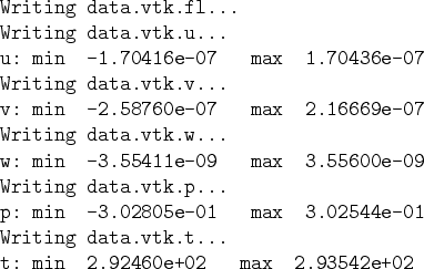
To visualize data using viewNaSt3DGP.tcl first create files in VTK-readable format using navsetup with the -G and -o $\langle$datafile$\rangle$ switch (this will create the files $\langle$datafile$\rangle$.vtk.p, $\langle$datafile$\rangle$.vtk.u, $\langle$datafile$\rangle$.vtk.v and so on, see section  for details). While converting the data navsetup will produce output which contains a passage similar to that in table .

Table: Sample output of navsetup while converting data.

Now you may use the command vtk viewNaSt3DGP.tcl $\langle$datafile$\rangle$ to start the Tk-based GUI (depending on the locations of your datafiles and viewNaSt3DGP.tcl you may have to supply appropriate paths to the above command). This will produce two windows on your screen (see figure ), the Tk-based GUI and the window into which VTK renders its output. Initially the render window will only show the bounding box of the data set (you can turn the bounding box on and off by clicking the button labeled ``Frame'').

Figure: The VTK render window and the viewNaSt3DGP GUI

Inside of the render window you can use the buttons of your mouse to rotate (left button), move (middle button/both buttons) and zoom (right button) the displayed object. The button labeled ``Exit'' of course ends the application. Clicking the button ``ppm'' will export the current content of the render window to a ppm file, the files will be named snapshot_1.ppm, snapshot_2.ppm and so on (Note, however, that the window content is not rendered off-screen, so e.g. overlapping windows or the mouse-pointer would also be exported to the ppm-file).

You can now add selected data using the two pulldown-menus on the top right of the GUI window. The menus ``Slice'' and ``IsoSurf'' are used to set the field variable which is to be displayed either on cut-planes (slices) or on an isosurface, respectively. In the entry field ``IsoSurfValue'' you have to enter the value for which the isosurface should be computed. With the button labeled ``On/Off'' you can toggle the isosurface. The two sliders are used to control the opacity of the isosurface and the displayed flag field (if there are obstacles in your data file). With the remaining buttons you can toggle the visibility of the cut-planes or move them through the domain. To adjust the color palette to the range of the displayed variable simply enter the appropriate maximum and minimum values into the correspondingly labeled fields.