Running a first example

In this section the general usage of the software package NaSt3DGP is shown, involving all the steps from generating an input file until visualising the final output. For detailed information on the usage of navsetup and navcalc/navcalcmpi please refer to the corresponding chapters of this manual. Both programs show a basic help message when called with the option -h.

First, choose a directory where you want to store and and work with the generated data, e.g. /home/my_home/Nast-Examples. Change to this directory and copy the file cavity.nav from PREFIX/share/licenses/nast3dgp/examples/Cavity2D into this directory. The format and all parameters of this file are described in detail in section . Now execute navsetup in the following way:

navsetup -s cavity.nav -b cavity.bin

Remark: Depending on the installation PREFIX you choose, you may have to call navsetup with the complete path, i.e. PREFIX/bin/navsetup or else include the directory PREFIX/bin into your PATH environment variable. This holds for all subsequent calls to binaries of the NaSt3DGP package.

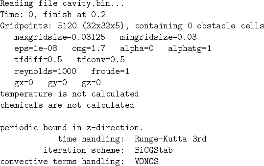
The setup program navsetup reads the configuration file cavity.nav which contains all necessary parameters for the description of the 'Driven Cavity'-testcase and generates a binary data file cavity.bin. This binary file contains all the data required for the subsequent computation with navcalc, i.e. the computational grid, initial values for ${\bf u}$ and $p$ and other necessary parameters. The generated binary file can be used for both serial and parallel computations.

To start the actual simulation, use the command

navcalc -b cavity.bin -p3

for the serial version and the following one for running a parallel calculation on 2 processors:

mpirun -np 2 navcalcmpi -b cavity.bin -p3

Remark: the actual command for running a parallel calculation may differ from the one above, depending on your installation of MPI.

Table: Sample output at startup of navcalc.

Table: Additional output of navcalcmpi.

The first calculation runs only for ten timesteps in order to get results quickly.

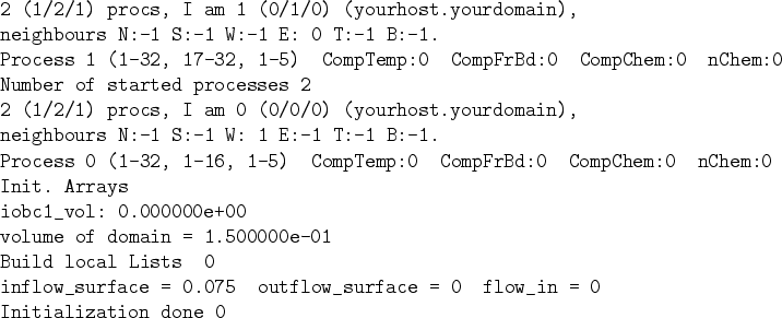
At the beginning, navcalc prints some information on the calculation it is about to perform, you can use this output to check if the most important parameters in the scene description file are set correctly. When running in parallel mode, additional output about the distribution on different processors/machines is displayed. Sample output looks similar to the one shown in tables  and .

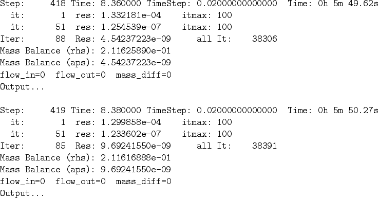
During the calculation navcalc prints some information on the screen(table ), e.g. the actual time, the size of the timestep, the divergence of the velocity field and information about the residuals of the pressure poisson equation.

Table: Runtime information of navcalc/navcalcmpi.

When the final time is reached, the data file cavity.bin is overwritten with the calculated data from the final time. The command

navsetup -TC cavity.bin -o results

generates a file named results.dat which is suitable for processing with Tecplot. The NaSt3DGP package supports several different output formats, e.g. for Matlab or VTK^2.1. For details about different data conversion possibilities of navsetup, refer to chapter .

The results for the first, very short simulation are shown in figures  and .

Figure: Contour lines of $u$,$v$ and $p$ (left to right) at time $t=0.1$.

Figure: Streamlines and velocity vectors at time $t=0.1$.

Now edit the scene description file cavity.nav and increase the simulation time by setting a value of 250 for Tfin. Rerun this example by following the steps above for the new cavity.nav file^2.2. Now the flof pattern does look like what you would expect for the 'Driven Cavity'-problem, since the solution has reached the steady state (see [1] or [4]). Visualizations of the result done with Tecplot are shown in figures  and .

Figure: Contour lines of $u$,$v$ and $p$ (left to right) in steady state (time $t=250$).

Figure: Streamlines and velocity vectors in steady state (time $t=250$).

More examples are presented in chapter . See section  for details on the format of the scene description file to design your own problem descrption files.