Next: Discretization of boundary conditions Up: Numerical Method Previous: Boundary conditions Contents
Computational grid and spatial discretization
In [1] only uniform grids were used.
Therefore we present the difference stencils used for the staggered grid.
A 2D example is shown in figure ![\includegraphics[width=0.6\textwidth,keepaspectratio]{p2.eps}](img72.png)
Velocity components and pressure values are defined on the nodes:
| defined on |
|
|
| `` |
|
|
| `` |
|
|
| `` |
|
|
|
|
`` |
|
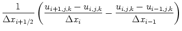
Diffusive terms:
![$\displaystyle \left[\frac{\partial^2 u}{\partial x^2}\right]_{i,j,k}$](img94.png) |
 |
||
![$\displaystyle \left[\frac{\partial^2 u}{\partial y^2}\right]_{i,j,k}$](img96.png) |
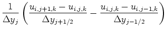 |
The other diffusive terms are discretized in a similar fashion. Stencils similar to the one for
Convective terms:
Five different discretizations of the convective terms are possible:
- Donor-Cell (hybrid-scheme) (1st/2nd order)
- Quadratic upwind interpolation for convective kinematics (QUICK) (2nd-Order)
- Hybrid-Linear Parabolic Arppoximation (HLPA) (2nd-Order)
- Sharp and Monotonic Algorithm for Realistic Transport (SMART) (2nd-Order)
- Variable-Order Non-Oscillatory Scheme (VONOS) (2nd/3rd-Order) (default)
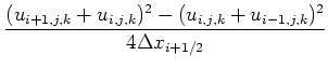
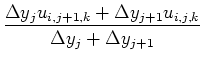
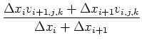
Second order convective terms:
![$\displaystyle \left[\frac{\partial u^2}{\partial x}\right]_{i,j,k}$](img103.png) |
 |
||
![$\displaystyle \left[\frac{\partial vu}{\partial y}\right]_{i,j,k}$](img105.png) |
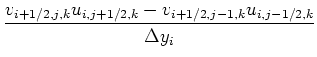 |
Stencils similar to the one for
![$\displaystyle \left[\frac{\partial vT}{\partial y}\right]_{i,j,k} = \frac{v_{i+1/2,j ,k} T_{i,j+1/2,k} -
v_{i+1/2,j-1,k} T_{i,j-1/2,k} }{\Delta y_{i }}\quad.
$](img108.png)
 |
|||
 |
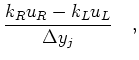
First order upwind:
|
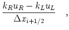 where where |
||
and 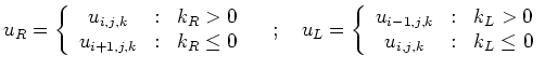 |
|||
|
 where where |
||
and 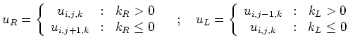 |
|||
Stencils similar to the one for
 first order
Laplacian for pressure:
We employ a conservative discretization which is simply the nested application of the centered difference for the pressure gradient and the centered difference for the natural discretization of the divergence, e.g.
![$\displaystyle \left[\frac{\partial^2 p}{\partial x^2}\right]_{i,j,k} =
\frac{1}...
...Delta x_{i+1/2}}-
\frac{p_{i,j,k}-p_{i-1,j,k}}{\Delta x_{i-1/2}}\right) \quad.
$](img123.png)
Poisson solvers:
For the solution of the linear equation arising from discretization of the pressure poisson equation, the following numerical methods are implemented:
- Successive Overrelaxation (SOR)
- Symmetric SOR (forward/backward)
- Red-Black scheme
- 8-Color SOR
- 8-Color Symmetric SOR (fw/bw)
- BiCGStab
To select a method, select the corresponding option in the scene
description file(see section ![]() on how to do this).
By default, the Poisson-equation is solved using the BiCGStab-method.
on how to do this).
By default, the Poisson-equation is solved using the BiCGStab-method.
Next: Discretization of boundary conditions Up: Numerical Method Previous: Boundary conditions Contents Martin Engel 2004-03-15